
Introduction#
Tech industry is on steroid with ml the development that took more than 10 yrs are happening less than a year because of AI and many stuff are taken as granted behaves as it is how it is supposed to be but I don’t want to take it as granted and as a black box i want to understand it all from the beginning.
Motivation#
I was semi unemployed and bored so i dedicated a week for ml to learn it all the way from linear regression to multimodal and state of the art,research on world models.This is my act to document stuff I still don’t have habit to document digitally I have a notebook documented and writing this after that week hope you will like it if not i don’t even care it’s for me bitch.
Linear Regression (1800)#
Linear Regression is simplest fundamental supervised learning algorithm used to model relation between dependent variables and one or more independent variables.The goal is to find the best fitting straight line or hyperplane that represents the association between these variables.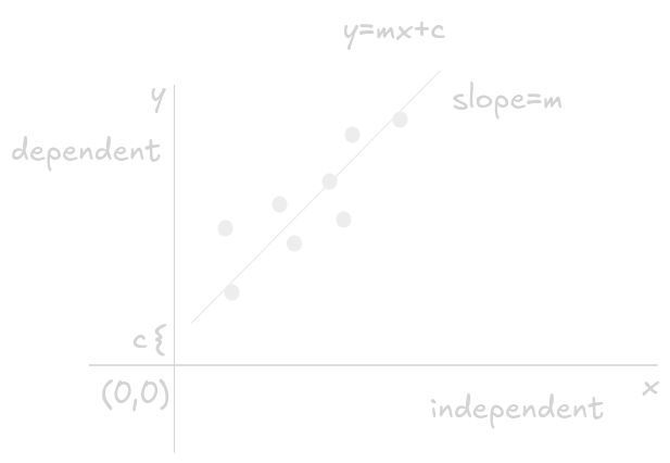
The training process looks like a random line is drawn and error is calculated MSE or RSS and we try to minimize error by changing slope and intercept according to error.
K-Nearest Neighbors (1951)#
K-Nearest Neighbor is another simplest supervised learning algorithm it is used for classification as well as regression,it’s lazy learner algorithm meaning it doesn’t actully learns it computes on inferece.
Main principle “If it quack and walk like duck it is a duck”.
KNN Classification → majority vote of nearest neighbors.
KNN Regression → average of nearest neighbors’ values.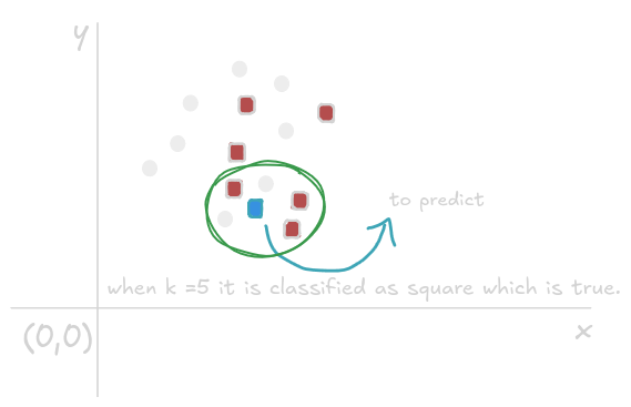
In above example k value was 5 what if k value was 3 it will be classified as circle false so value of k is hyperparameter and tuned according to data during validation step.Other use case is clustering using distance matrix.
Perceptron (1958)#
A Perceptron is one of the simplest forms of an artificial neuron and is commonly used for binary classification.It is used when data is linearly separable using a line.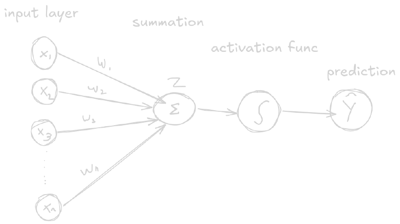
How Does a Perceptron Learn?#
Unlike KNN, which mainly stores the training data, a perceptron actually learns parameters.
During training, it learns:
- The weights $algorithmw_i$
- The bias $b$
1. Compute the Weighted Sum#
$$ z = \sum_{i=1}^{n} w_i x_i + b $$
2. Apply the Step Function#
$$ \hat{y} = \begin{cases} 1 & \text{if } z \geq 0 \ 0 & \text{otherwise} \end{cases} $$
3. Calculate the Error#
$$ \text{error} = y - \hat{y} $$
4. Update the Weights#
$$ w_i \leftarrow w_i + \eta (y - \hat{y})x_i $$
where $\eta$ is the learning rate.
5. Update the Bias#
$$ b \leftarrow b + \eta (y - \hat{y}) $$
6. Repeat for Multiple Epochs#
The perceptron processes the training dataset repeatedly.
One complete pass through the entire training dataset is called an epoch.
Naive Bayes (1960)#
Also supervised learning algorithm based on Bayes theorem. Here, Naive means every variable used is independent.
Bayes’ theorem describes how we update the probability of an event when we obtain new evidence.
The formula is:
$$ P(A \mid B) = \frac{P(B \mid A)P(A)}{P(B)} $$
Where:
$P(A \mid B)$ — probability of $A$ given $B$ (posterior)
$P(B \mid A)$ — probability of $B$ given $A$ (likelihood)
$P(A)$ — probability of $A$ before observing the evidence (prior)
$P(B)$ — probability of observing $B$ (evidence)
With conditional independence assumption (Naive Bayes):
$$P(A|B,C,D,E,\ldots,N) = \frac{P(B|A) \cdot P(C|A) \cdot P(D|A) \cdot P(E|A) \cdots P(N|A) \cdot P(A)}{P(B,C,D,E,\ldots,N)}$$
Example#
| Person | COVID (Yes/No) | Flu (Yes/No) | Fever (Yes/No) |
|---|---|---|---|
| 1 | Yes | No | Yes |
| 2 | No | Yes | Yes |
| 3 | Yes | Yes | Yes |
| 4 | No | No | No |
| 5 | Yes | No | Yes |
| 6 | No | No | Yes |
| 7 | Yes | No | Yes |
| 8 | Yes | No | No |
| 9 | No | Yes | Yes |
| 10 | No | Yes | No |
Step 1: Prior Probability#
$$P(\text{fever} = \text{yes}) = \frac{7}{10}$$
$$P(\text{fever} = \text{no}) = \frac{3}{10}$$
Step 2: Conditional Probability#
How to observe is example for 1st cell we see covid yes and fever yes 2nd cell covid yes fever no and divide them by total no of yes and no in data.
| Yes | No | |
|---|---|---|
| COVID | $\frac{4}{7}$ | $\frac{1}{3}$ |
| Flu | $\frac{3}{7}$ | $\frac{1}{3}$ |
Bayes’ Theorem Formulas#
Given Person (Flu, COVID):
$$P(\text{Fever = Yes} \mid \text{Flu, COVID}) = P(\text{Flu} \mid \text{Yes}) \cdot P(\text{COVID} \mid \text{Yes}) \cdot P(\text{Yes})$$
$$= \frac{3}{7} \times \frac{4}{7} \times \frac{7}{10} = \frac{84}{490} = 0.171$$
$$P(\text{Fever = No} \mid \text{Flu, COVID}) = P(\text{Flu} \mid \text{No}) \cdot P(\text{COVID} \mid \text{No}) \cdot P(\text{No})$$
$$= \frac{1}{3} \times \frac{1}{3} \times \frac{3}{10} = \frac{3}{90} = 0.033$$
So here probability of person having fever is more than not having fever when having covid and flu so it’s classified as fever.
Backpropagation (1986)#
Lets take an example of Multi layer perceptron as.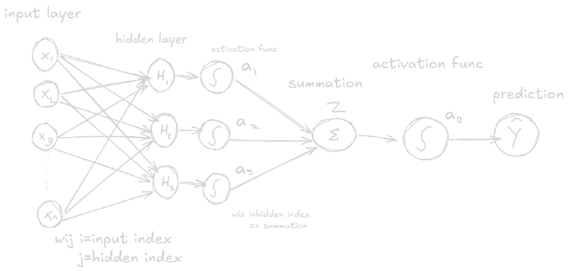
How does it learn is Backpropagation it’s is the algorithm neural networks use to learn by adjusting weights to reduce prediction errors. It works backwards through the network, calculating how much each weight contributed to the error.
The core idea is
- Forward Pass: Data flows through network → prediction
- Calculate Error: Compare prediction to actual answer
- Backward Pass: Error flows backwards → calculate how much to fix each weight
- Update Weights: Adjust weights to reduce error
The Chain rule:#
The chain rule tells you how to find the total effect when something changes through multiple steps.
In one sentence: If A affects B, and B affects C, then the total effect of A on C = (effect of A on B) × (effect of B on C) Lets take a component from our MLP, lets see how weight $w_1z$ affects cost function.
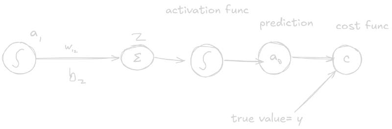
The cost depends on w₁z through this path: w₁z → z → a₂ → a₀ → C
$$\frac{\partial C}{\partial w_{1z}} = \frac{\partial C}{\partial a_0} \cdot \frac{\partial a_0}{\partial z} \cdot \frac{\partial z}{\partial w_{1z}}$$
Each term:
- $\frac{\partial z}{\partial w_{1z}} = a_1$ (because $z=w_1z*a_1+b_z$)
- $\frac{\partial a_0}{\partial z} = \sigma’(z)$ (activation slope)
- $\frac{\partial C}{\partial a_0} = 2(a_0 - y)$ (because $C=(a_0-y)^2$)
Final gradient:
$$\frac{\partial C}{\partial w_{1z}} = (a_0 - y) \cdot \sigma’(z) \cdot a_1$$
We can apply chain rule according to bias and take out gradient in respect for it.
Similarly we can derive for $w_11$ Let’s take component.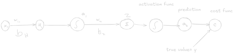
Decision Trees (1986)#
A decision tree is a method to make decision based on statement at parent node.If decision tree classifies thing it’s called classification tree else if it predicts value it’s regression tree.
Example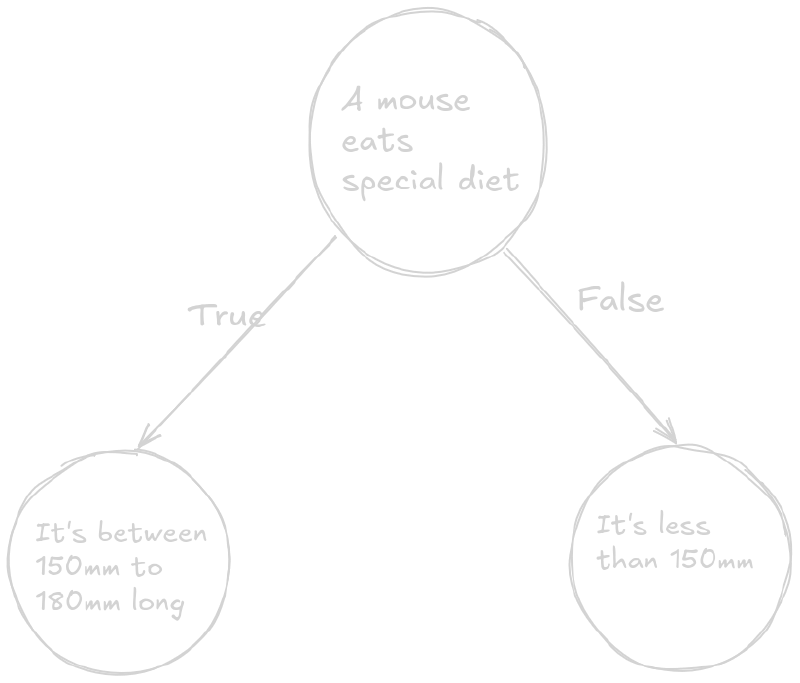
How to make decisiontree or how does it learn#
There is a problem on which feature to split first or last there are different ways to do that some of them are:
- Information Gain (Entropy) - Measures entropy reduction
- Gini Gain (Gini Index) - Measures impurity reduction
- Gain Ratio - Corrects for features with many values
- Chi-Square Test - Tests statistical significance
- Variance Reduction - For regression trees
Formulas#
| Metric | Formula |
|---|---|
| Information Gain | $IG(D,A) = Entropy(D) - \sum_v \frac{|D_v|}{|D|} Entropy(D_v)$ |
| Gini Gain | $GiniGain(D,A) = Gini(D) - \sum_v \frac{|D_v|}{|D|} Gini(D_v)$ |
| Gain Ratio | $GR(D,A) = \frac{IG(D,A)}{SplitInfo(D,A)}$ |
| Chi-Square | $\chi^2 = \sum_{i,j} \frac{(Observed - Expected)^2}{Expected}$ |
| Variance Reduction | $VR(D,A) = Var(D) - \sum_v \frac{|D_v|}{|D|} Var(D_v)$ |
Example: Finding the Root Node Using Information Gain#
| Outlook | Temperature | Humidity | Windy | Play? |
|---|---|---|---|---|
| sunny | hot | high | false | No |
| sunny | hot | high | true | No |
| overcast | hot | high | false | Yes |
| rain | mild | high | false | Yes |
| rain | cool | normal | false | Yes |
| rain | cool | normal | true | No |
| overcast | cool | normal | true | Yes |
| sunny | mild | high | false | No |
| sunny | cool | normal | false | Yes |
| rain | mild | normal | false | Yes |
| sunny | mild | normal | true | Yes |
| overcast | mild | high | true | Yes |
| overcast | hot | normal | false | Yes |
| rain | mild | high | true | No |
Summary: 14 total, 9 Yes, 5 No
Step 1: Calculate Initial Entropy#
$$Entropy(D) = -\frac{9}{14}\log_2\left(\frac{9}{14}\right) - \frac{5}{14}\log_2\left(\frac{5}{14}\right)$$
$$= -0.643(-0.644) - 0.357(-1.485) = 0.94 \text{ bits}$$
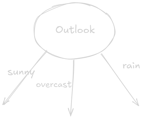
Step 2: Try Splitting on “Outlook”#
Sunny (5 records): 2 Yes, 3 No#
$$Entropy(Sunny) = -\frac{2}{5}\log_2\left(\frac{2}{5}\right) - \frac{3}{5}\log_2\left(\frac{3}{5}\right) = 0.971$$
Overcast (4 records): 4 Yes, 0 No#
$$Entropy(Overcast) = 0 \text{ (Pure!)}$$
Rain (5 records): 3 Yes, 2 No#
$$Entropy(Rain) = -\frac{3}{5}\log_2\left(\frac{3}{5}\right) - \frac{2}{5}\log_2\left(\frac{2}{5}\right) = 0.971$$
Step 3: Calculate Information Gain#
$$IG(Outlook) = Entropy(D) - \left[\frac{5}{14}(0.971) + \frac{4}{14}(0) + \frac{5}{14}(0.971)\right]$$
$$= 0.94 - 0.694 = 0.246$$
Step 4: Compare with Other Features#
| Feature | Information Gain |
|---|---|
| Outlook | 0.246 |
| Humidity | 0.151 |
| Windy | 0.049 |
| Temperature | 0.029 |
Result#
The root node should split on “Outlook” because it has the highest information gain (0.246).
Support Vector Machine (1992-1995)#
Support Vector Machine(SVM) is another supervised learning technique for classification and regression task.It tries to find the best hyperplane that separates different classes in the data.The main goal of SVM is to maximize the margin between the two classes. The larger the margin the better the model performs on new and unseen data.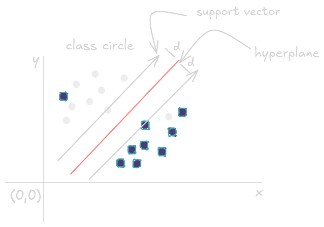
If data is not linearly separatable we use kernel to map then in higher dimenstion space and then use svm
Bagging (1994)#
Is Parallel Ensemble learning technique.Bagging or Bootstrap Aggregating, the idea is to traing multiple base models independently and in parallel on different bootstrapped sample of the training data and Aggregate them.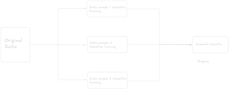
Boosting (1995)#
Boosting is a sequential ensemble learning technique.It is a process that uses a set of machine learning algorithms to combine weak learner to form strong learners in order to increase the accuracy of the model.
The basic principle behind boosting is to generate multiple weak learners and combine heir prediction to form one strong rule.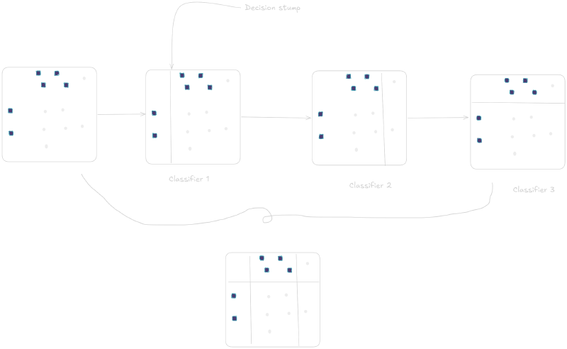
Recurrent Neural Network (1986)#
We saw Neural networks for constant size of input but what if input is variable size like time series data(eg stock data,power consumption etc).In this cases we use Recurrent Neural Networks.
RNN architecture#
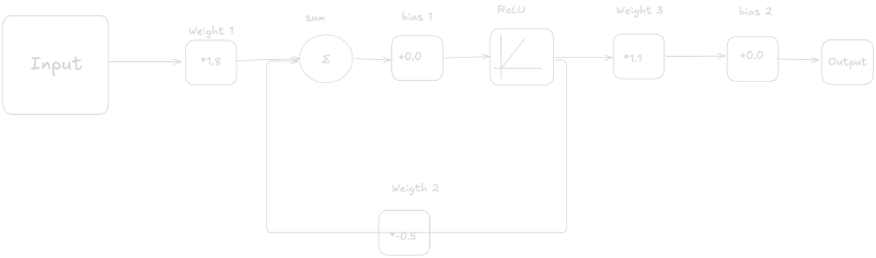
Although the development it is not used widely because of the problem called vanishing gradient. When we unroll the rnn more it causes vanishing of gradient while backpropagaton
RNN unrolling (Vanishing/Exploding Gradient)#
RNN are unrolled as follow when data ingestion during training or inference.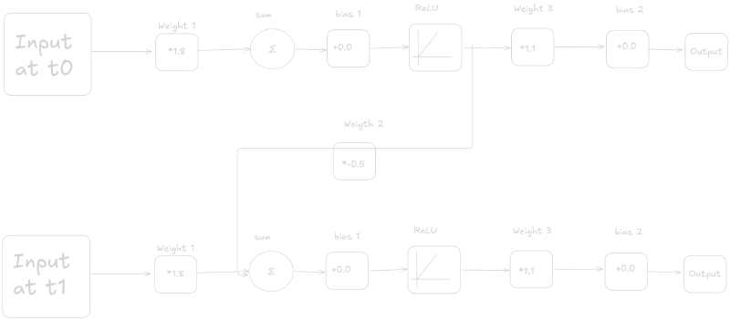
While backpropagaton we multiply weight each time in gradient and if it is < 1 it shrink every time and vanishes if unrolled too much.
Why the term $W_2$ comes in multiply because as in chain rule we take partial diff of summations during unrolling with respect to $W_1$ or layer 1 term and we have $W_1$ terms whose diff is 1 and $W_2$ comes on gradient due to chain rule.Similarly if the weight in unrolling step is greater than 1 it causes exploding gradient.
Long Short Term Memory (1997)#
To solve vanishing gradient problem there comes LSTM(Long Short Term Memory).LSTM is a type of RNN.LSTM uses two paths to make prediction one for long term and other for short term.
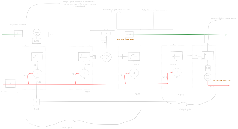
It’s complicated i know but take it one layer at a time and you will get it. The input gate is to determine the long term memory and output gate is to determine short term memory there are two activation function sigmoid and tanh used for different cases.
LSTMs are also unrolled for time varying data or data having variables input size.
Random Forests (2004)#
Random forests is one of the bagging method(parallel ensemble learning) where we create bootstrapped dataset and then create decision tree using that bootstrapped data, we repeat these steps multiple times and vote for out while inference. Building decision tree is explained above and also bagging.
For evaluation we use out of bag sample.
Also we can change the number of variables used per step and build random forest evaluate it and then use the one with highest accuracy.
Random forest can also be used for missing value and clustering.
Gradient Boosting Machine (2001)#
It is one of the type of Boosting expalined above.In gradient boosting base learners are generated sequentially in such a way that the present base learner is always more effective than previous one. We optimize the loss function of the previous learner.
The 3 components here are :
- Loss function needs to be minimized
- Weak learner for prediction and forming then strong.
- Additive model for regularizing loss function.Regularizing loss function means adding an extra penalty to the normal loss so the model is discouraged from becoming unnecessarily complex or having very large weights.
Restricted Boltzmann Machine (2002)#
It it probabilistic unsupervised learning technique mostly used in case of recommendation system.
It has two layer visible and hidden and they are fully connected trains like regular mlp.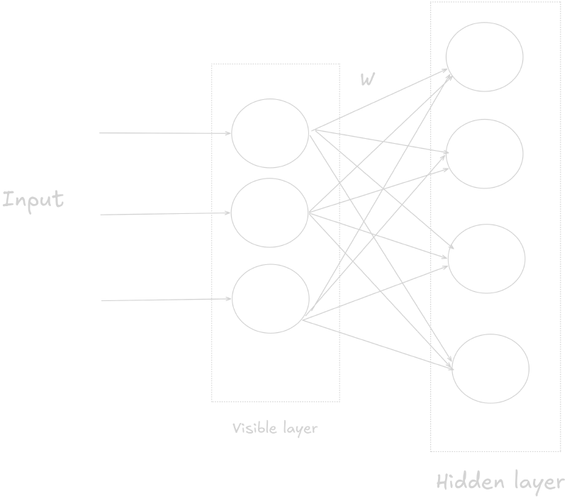
Deep Belief Network (2006)#
It is a composition of stack of unsupervised networks such as Restricted Boltzmann Machine.
The hidden layer in stack first is the visible layer fore the stack second.
Deep Belief Network has connections with RBM and not between RBMs.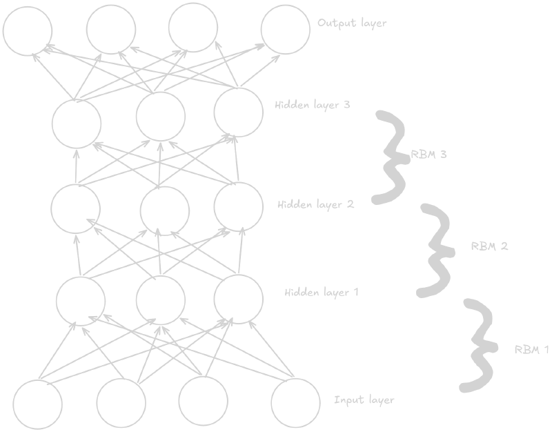
CNNs (1998)#
CNNs were introduced by Yann LeCun through famous LeNet-5.The need of CNN can be explained as follow
- In fully connected network the connections becomes complex and computationally inefficient because of enormous image size
- A fully connected network doesn’t naturally understand that nearby pixels are related.
High level design of Convolution on Neural Nets#

Components of CNNs#
Padding#
As the edge can contribute less to feature as they will be used once only while shifting filter we use padding adding extra layer of pixel usually 0.
Stride#
Stride mean what step filter takes while moving both horizontally and vertically.
Filters#
Filters are used for different purpose like edge detection,blur,sharpen,gaussian blue etc and they are also learned during training process.
Input Image (6×6)
| 10 | 20 | 30 | 40 | 50 | 60 |
| 15 | 25 | 35 | 45 | 55 | 65 |
| 20 | 30 | 40 | 50 | 60 | 70 |
| 25 | 35 | 45 | 55 | 65 | 75 |
| 30 | 40 | 50 | 60 | 70 | 80 |
| 35 | 45 | 55 | 65 | 75 | 85 |
Filter (3×3)
| -1 | 0 | 1 |
| -2 | 0 | 2 |
| -1 | 0 | 1 |
Output (4×4)
Input * filter=
| 80 | 80 | 80 | 80 |
| 80 | 80 | 80 | 80 |
| 80 | 80 | 80 | 80 |
| 80 | 80 | 80 | 80 |
Formula For Output Height and Width#
$$N_{out,h} = \left\lfloor \frac{N_{in,h} - F_h + 2P}{S} \right\rfloor + 1$$
$$N_{out,w} = \left\lfloor \frac{N_{in,w} - F_w + 2P}{S} \right\rfloor + 1$$
where F is Filter size, S is Stride size, P is No of layer of Padding
Polling Layer#
It is a way to reduce the spatial size of feature maps while keeping the most important information. Mainly of 2 types Max Polling and Average Polling.
Input matrix#
| 8 | 5 | 6 | 2 |
| 3 | 9 | 1 | 4 |
| 7 | 2 | 8 | 5 |
| 1 | 6 | 3 | 9 |
Pool size 2 by 2 and stride of 2
Output matrix#
| 9 | 6 |
| 7 | 9 |
Output size#
$$N_{out,h} = \left\lfloor \frac{N_{in,h} - F_h}{S} \right\rfloor + 1$$
$$N_{out,w} = \left\lfloor \frac{N_{in,w} - F_w}{S} \right\rfloor + 1$$
Padding is not used in pooling generally.
AlexNet (2012)#
One of the Famous architecture based on CNNs It has 8 layers and nearly 60M parameter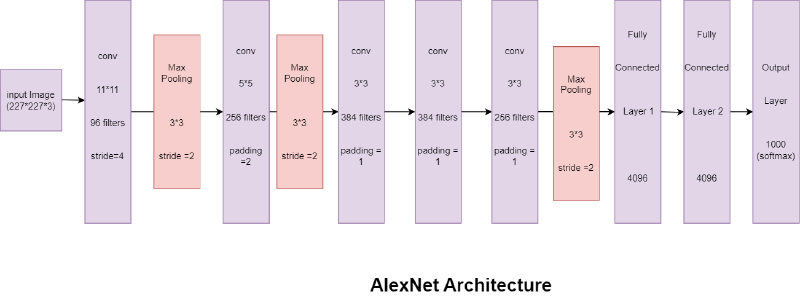
Word2Vec and GloVe(2013-2014)#
Word2Vec is a neural network-based method that learns word embeddings from large text corpora. Developed by Google in 2013.
Main idea: A word is best understood by the company it keeps (context words around it).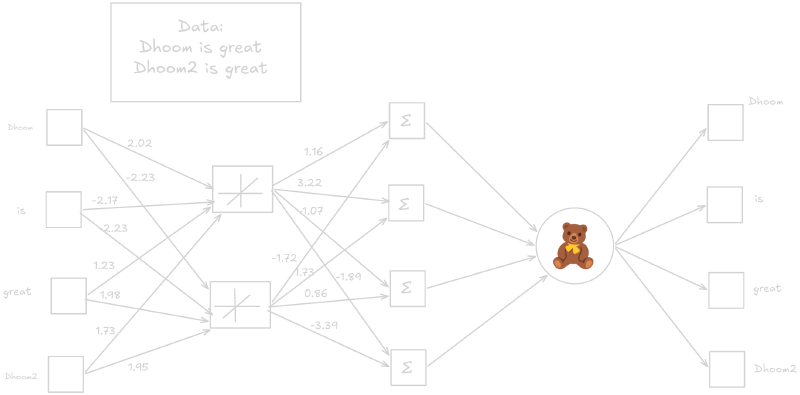
So the training process is like we assign 1 to first word and we want network to predict the second word if not we calculate cost using cross entropy loss and adjust weight throught backpropagation.
This step is followed for each word to predict next word now after training the weight on first layer gives its vector embeddings.Also it’s not teddy bear it’s softmax ha ha.
After training we see.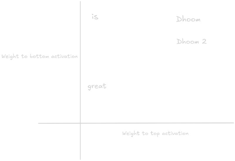
GloVe stands for Global Vector.GloVe is a matrix factorization-based method that combines:
- Global matrix factorization (captures global statistics)
- Local context windows (captures local context)
Data#
Sentence 1: I love physics Sentence 2: I love geeking
Vocabulary: [I, love, physics, geeking]
Window Size = 1#
Co-occurrence Matrix#
| I | love | physics | geeking | |
|---|---|---|---|---|
| I | 0 | 2 | 0 | 0 |
| love | 2 | 0 | 1 | 1 |
| physics | 0 | 1 | 0 | 0 |
| geeking | 0 | 1 | 0 | 0 |
Matrix Factorization#
$$X \approx WC^T$$
Where $W$ contains word vectors (reduced to 2 dimensions): We first randomly assign W and C and try to predict X co-occurrence matrix calcuate error and fix our matrix.
| Word | Vector |
|---|---|
| I | $[0.48, 0.52]$ |
| love | $[0.72, 0.75]$ |
| physics | $[0.71, 0.74]$ |
| geeking | $[0.70, 0.73]$ |
Key Observation#
physics and geeking have identical co-occurrence patterns → similar vectors
Because both appear only with love in window of 1.
The Intuition#
$$\text{Text} \rightarrow \text{Co-occurrence} \rightarrow \text{Matrix} \rightarrow \text{Factorization} \rightarrow \text{Embeddings}$$
A word’s meaning is learned from the company it keeps.
VGG16 and GoogleNet (2014)#
They are CNN based architecture VGG16 has 16 layers and about around 138 M parameters .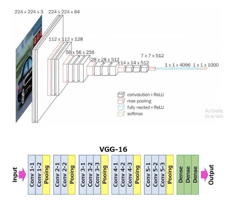
Sequence to Sequence (2014)#
Sequence to Sequence is Encoder Decoder based Neural Net. Internally it uses LSTM heavely insider encoder and decoder stack. Used in translation and stuffs.In our example we will see english to spanish translation.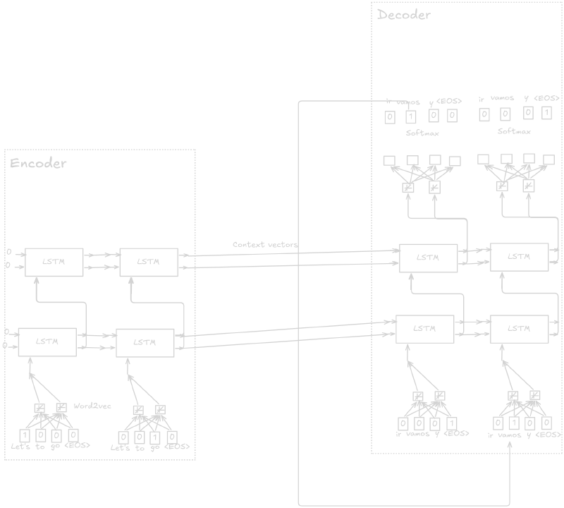
Teacher Forcing#
Plugging in the known words and stopping at the known phrase length, rather thean using predicted token for everything if wrong.
Attention (2015)#
Problem with seq2seq is unrolling the LSTMs compresses the entire input sentence into single context vector, it forgets word inputted early on for say 1000 page doc and so.
So the main idea of attention is to add a bunch of new paths from the encoder to the decoder,one per input value,so that each step of the decoder can directly access input values.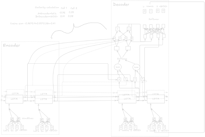
ResNet (2015)#
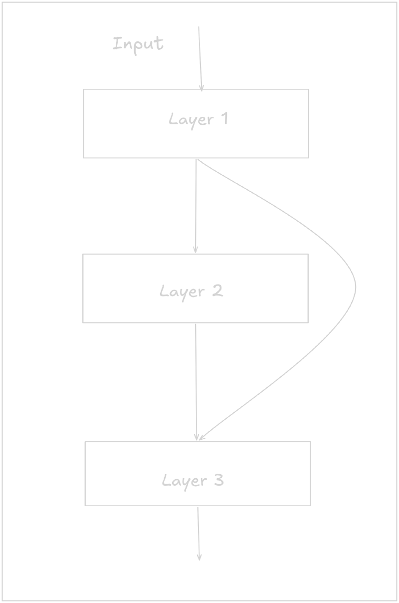
- It it a type of CNN containing 152 layers(approx) overcomes vanishing gradient due to grawth of CNNs
- ResNet include “skip connection” feature which enables training of multiple deep layers(152 layers) without vanishing gradient issues.
XGBoost (2014)#
Advance version of Gradient boosting method that is designed to focus on computaional speed and model efficiency.Supports distributed computation,out of core computing,parallelization,cache optimization
Transformer “Attention is all you need” (2017)#
Architecture#
It is neural network with different mechanism to understand properly.Also it contains encoder decoder stack.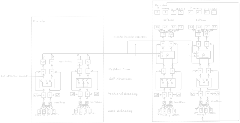
Components#
Word Embeddings#
I won’t talk much just to represent word to number read above in its section.
Positional Encoding#
Position of word matters in sentences like “I eat chicken” and “Chicken eat me” they have same words but completely different meaning so we need to use unique number to represent words position which is done by sine and cosine squiggle alternatively.
Self Attention#
With self attention we calculate similarity of a word with itself and other Its value Query,key and value are calculated from multiplying the word embedding + Positional encoding with weights.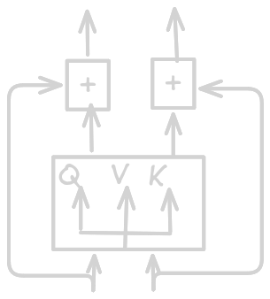
Residual connection#
Ther self attention value is again added with word embedding+positional embedding the connection is called connection residual connection.It is useful because:
- It prevents information Loss
- It makes learning an identity function easy
- It helps gradients flow through deep Transformers
Encoder Decoder Attention#
Same like self attention mechanism but we take value and key from encoders and query from decoder and calculate similarity and which give word that has more context and in our example which to translate first.
In paper “Attention is all you need” stack of 8 self attention was used.
BERT “Encoder only transformer” (2018)#
- Encoder only Transformers.
- It helps cluster similar sentences or even documents.
- Only use self attention and can create Context aware embedding.
- The ability to cluster similar sentences and documents is the foundation for something called Retrieval Augumented Generation or RAG.
- Other cool usecase can be sentiment analysis.
Training#
While training it goes througt 3 passes each of:
- Pretraining to understand language
- Fine tuining to learn specific task.
GPT series “Decoder only transformer” (2018 onward)#
- Decoder only Transformer
Training#
It uses transfer learning technique
- Pretraining: Train the GPT arch to understand what language is
- Finetuning: Uses transfer learning to make GPT architecture perform well on specific task(Transferring knowledge)
Problem with fine tuining#
- Still too much data required.
- Overfitting is easy.
- Not how human learns.
- Not fluid to understand broad language processing.
Meta learning#
- Zero Shot learning It was introduced in GPT2 perform specific task when given just an instruction and input.
- One shot learning Giving 1 example.
- Fwe shot learning Giving multiple example.
GPT 3 used all of this learning technique.
Diffusion Model (2015 theory,2020 practical products)#
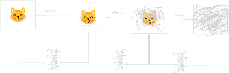
Diffusion models are generative model used for images generation video generation an so on. It really mathematically heavy I will understand it more and write about it in future.
CLIP (By openai)#
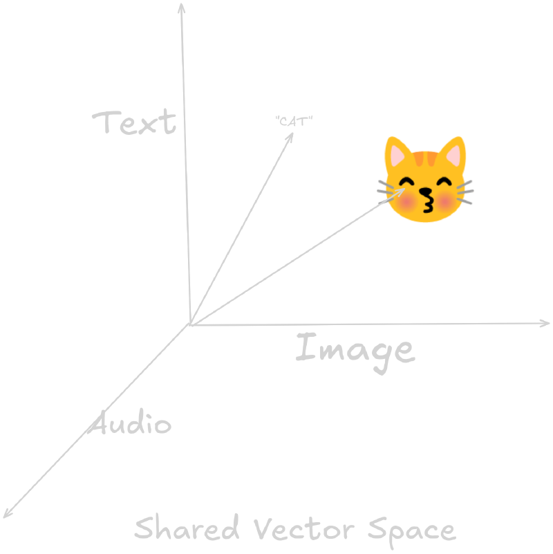
CLIP Contrastive Language-Image Pre-Training is model by openai whic contains image encoder and text encoder and image with their caption lies close in multi dimensional space I mean a image embedding and it’s caption text embedding.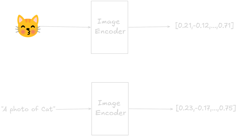
General Algorithm for Training Diffusion models#
Multimodal Models (2020)#
- Here in multimodal modal refers different data modality.
- Different technique were used to support multimodal some are:
- Feature level fusion
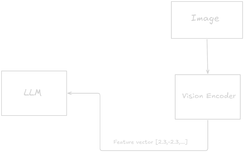
- Native Multimodality
Lightweight Distillation,quantization(2020)#
Distillation#
The process of transferring knowledge from a larger often more complex model refered to as the teacher to a similar more efficient model.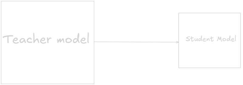
Quantization#
Is the process of mapping input value from a large set of output value in as smaller set.Reducing the precision of weight value in neural nets.Also the activation function. Example reducing from FP32 to INT8.One cool engineering project using it is Airllm
World Model and JEPA (2022)#
LeCun’s Philosophy “Real Intelligence does not start in language. It starts in the world.” Development of JEPA follows the usage of multiple stepping stones like Siamese Network,Representation collapse,Barlow Twins.
World Model let’s put it in this way common sense can be seen as a collection of models of the world that can tell an agent what is likely,what is plausible and what is impossible.Using such models, we can learn new skills with very few trials. We can predict consequences, reason and plan.
JEPA stands for Joint Embedding Predictive Architecture.
As the name suggest we observe environment at time x(t) pass it through encoder for embedding and try to predict embedding at x(t+1) also observe at x(t+1) and try to minimize prediction error. In this process the network learn the world model.Eg trying to predict what comes next in dash cam of camera.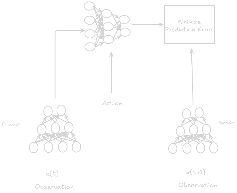
V-JEPA and VLM(Vison Language Models) and VLA(Vision Language Action) and VL-JEPA#
LeCun puts an interesting idea “How can an agent perform task if it doesn’t know the consequences of it’s action?”
He says the JEPA will be developed for different task than llm like vision stuffs physical intelligence and slowly it will replace llm he says we achieved intelligence in language first which is not natural like in human we achieve it in vision or on experience(eg gravity touch and so).
V-JEPA and VLM#
Both are made to understand image and video properly.CLIP from openai is example of VLM.In V-JEPA the network doesn’t learn anything about language just visuals. JEPA/VL-JEPA research has demonstrated strong parameter/data efficiency in specific controlled benchmarks, while V-JEPA itself is primarily a visual representation/world-modeling approach rather than a direct VLM competitor.
Problem with VLA#
- Difficulty of scaling behavior cloning
- Lack of explicit planning
Both are tried to be solve by world model.